Finding rare (un-annotated) cell types with DRVI

Rare cell types / states are often missing from the annotations of a dataset: there are too few of them to form their own cluster, so they get absorbed into a neighboring cell type’s label. DRVI, however, tends to give such a population its own latent dimension, because the population has a distinct gene program.

In this notebook we define a rare-cell-type dimension by three criteria and use them to scan the DRVI latent space of the immune dataset:

1. Rare activity — Only a small fraction of cells are active on the dimension.

2. Spatial cohesion — The active cells sit close together in the latent manifold, rather than being scattered.

3. Interpretability — The dimension has a significant gene program signature.

The immune dataset (human PBMC / bone marrow) has no Fibroblast annotation. Yet a handful of fibroblast contaminant cells are present. We will discover them as a dimension that meets the three criteria, use the interpretability scores to hypothesize their identity, and finally prove it with the canonical fibroblast marker COL1A1 — a gene that was not among the 2000 highly variable genes (HVGs) the model was trained on, but is present in the full data.

We reuse the already-trained model from the general DRVI pipeline — there is no retraining here.

Contact

For questions and help requests, you can reach out in the scverse discourse.

If you found a bug, please use the issue tracker.

Install

This notebook uses the tutorials extra of drvi-py (DRVI plus helper packages such as leidenalg, used here for Leiden clustering). Install it once in your environment with:

pip install "drvi-py[tutorials]"

On Colab, the next cell does this for you. Remove it if your environment is already set up.

import sys
import subprocess

# if branch is stable, will install via pypi, else will install from source
branch = "latest"
IN_COLAB = "google.colab" in sys.modules

if IN_COLAB and branch == "stable":
    subprocess.check_call([sys.executable, "-m", "pip", "install", "drvi-py[tutorials]"])
elif IN_COLAB and branch != "stable":
    subprocess.check_call([sys.executable, "-m", "pip", "install",
                           "git+https://github.com/theislab/drvi.git#egg=drvi-py[tutorials]"])

Imports

import warnings
warnings.filterwarnings("ignore")

from pathlib import Path

import numpy as np
import pandas as pd
import anndata as ad
import scanpy as sc

from scipy.spatial.distance import pdist

import scvi
import drvi
from drvi.model import DRVI

print("Last run with scvi-tools version:", scvi.__version__)
print("Last run with DRVI version:", drvi.__version__)

Last run with scvi-tools version: 1.4.3
Last run with DRVI version: 0.2.6

# Making plots prettier
sc.set_figure_params(dpi=100, frameon=False, figsize=(3, 3))

from matplotlib import pyplot as plt
plt.rcParams["figure.dpi"] = 100
plt.rcParams["figure.figsize"] = (3, 3)

Config

We load the artifacts produced by the general training/interpretability pipeline:

• drvi_model — the trained DRVI model.

• embed.h5ad — the latent space (one column per latent dimension) with dimension stats in embed.var and pre-computed interpretability scores in embed.varm.

• Immune_HVG_human.h5ad — the counts (2000 HVGs) the model was trained on, from the scverse example data server.

• Immune_ALL_human.h5ad — the full gene set from the scverse example data server (used only at the end to validate with the held-out marker).

io_dir = Path("./tmp_io/drvi_immune_128/")

embed_path = io_dir / "embed.h5ad"
adata_path = io_dir.parent / "Immune_HVG_human.h5ad"
model_path = io_dir / "drvi_model"
full_anndata_path = io_dir.parent / "Immune_ALL_human.h5ad"

# Column in `embed.obs` / full data holding the existing cell-type annotation.
CELL_TYPE_COL = "final_annotation"

# Thresholds defining a rare-cell-type dimension (see the three criteria above).
ACTIVITY_FRACTION = 0.5    # a cell is "active" if |latent| exceeds this fraction of the dimension's peak |latent|
MAX_RARE_FRACTION = 0.01   # a dimension is "rare" if fewer than this fraction of cells are active
MIN_COHESION = 0.5         # min UMAP cohesion (1 = tight blob, ->0 = spread across the UMAP)
MIN_OOD_SCORE = 1.0        # minimum interpretability score for a gene program
HOST_COVERAGE_CUTOFF = 0.30  # a candidate "needs refinement" if it captures less than this share of its host label

Load artifacts

embed = sc.read_h5ad(embed_path)
adata = sc.read(
    adata_path,
    backup_url="https://exampledata.scverse.org/scvi-tools/Immune_HVG_human.h5ad",
)
embed

AnnData object with n_obs × n_vars = 32484 × 128
    obs: 'batch', 'chemistry', 'data_type', 'dpt_pseudotime', 'final_annotation', 'mt_frac', 'n_counts', 'n_genes', 'sample_ID', 'size_factors', 'species', 'study', 'tissue', '_scvi_batch', '_scvi_labels'
    var: 'original_dim_id', 'reconstruction_effect', 'order', 'max_value', 'mean', 'min', 'max', 'std', 'std_abs', 'title', 'vanished', 'vanished_positive_direction', 'vanished_negative_direction'
    uns: 'neighbors', 'pca', 'umap'
    obsm: 'X_pca', 'X_umap'
    varm: 'IND_exp_weighted_mean_negative', 'IND_exp_weighted_mean_positive', 'IND_linear_weighted_mean_negative', 'IND_linear_weighted_mean_positive', 'IND_max_negative', 'IND_max_positive', 'OOD_combined_negative', 'OOD_combined_positive', 'OOD_max_possible_negative', 'OOD_max_possible_positive', 'OOD_min_possible_negative', 'OOD_min_possible_positive', 'PCs'
    obsp: 'connectivities', 'distances'

# Set up and load the trained model. We only need it for the convenience interpretability API
# (get/plot_interpretability_scores); all three criteria are computable from `embed` alone.
DRVI.setup_anndata(
    adata,
    layer="counts",
    batch_key="batch",
    is_count_data=True,
)
model = DRVI.load(model_path, adata)
model

INFO     File tmp_io/drvi_immune_128/drvi_model/model.pt already downloaded
INFO     DRVI: The model is trained with DRVI version 0.2.6.
INFO     DRVI: Updaging data setup config ...
INFO     DRVI: Done updating data source registry. Loading in DRVI version 0.2.6.
INFO     DRVI: Loading model from DRVI version 0.2.6.
INFO     DRVI: Done updating model args. Loading in 0.2.6.
INFO     DRVI: The model has been initialized

DRVI 
Latent size: 128, splits: 128, pooling of splits: 'logsumexp', 
Encoder dims: [128, 128], 
Decoder dims: [128, 128], 
Gene likelihood: pnb, 

Training status: Trained

Scan every dimension for the three criteria

A few practical points:

• DRVI dimension titles do not match the column order in embed (e.g. DR 1 is not the first column), so we always index dimensions by their title.

• We read interpretability through the model interface, model.get_interpretability_scores(embed, adata). It returns a genes × dimensions table whose columns are the non-vanished signed dimensions (e.g. DR 1+).

# Set title as index for easier access to latent dimensions by name
embed.var.set_index("title", inplace=True, drop=False)

Utils for criterion 1: number of active cells in a dimension

def active_mask(embed, dim_title_direction):
    """Boolean mask of cells active on a given dimension/direction.

    The threshold is adaptive per dimension: a cell is active when its latent value passes half of
    the dimension's peak activation (`max(|latent|) * ACTIVITY_FRACTION`) in the requested direction.
    """
    dim_title = dim_title_direction[:-1]                  # e.g. "DR 49+" -> "DR 49"
    direction = dim_title_direction[-1]                   # e.g. "DR 49+" -> "+"
    column = np.asanyarray(embed[:, dim_title].X).flatten()
    cutoff = np.abs(column).max() * ACTIVITY_FRACTION     # per-dimension: max(|latent|) / 2
    return column > cutoff if direction == "+" else column < -cutoff

Utils for criterion 2: spatial cohesion (UMAP compactness vs Leiden clusters)

A real rare cell type forms a single tight blob rather than being scattered. We measure this directly on the 2-D UMAP — the space we actually visualize. We cluster the latent space with Leiden and take the typical within-cluster pairwise UMAP distance as a reference scale, then compare it to the spread of each dimension’s active cells on the UMAP:

cohesion = reference_cluster_scale / (reference_cluster_scale + median_pairwise_umap_distance_of_active_cells)

This is ~1 for a tight blob and drops toward 0 as the active cells spread out.

sc.tl.leiden(embed, resolution=1.0, key_added="leiden", flavor="igraph", n_iterations=2, directed=False)
leiden_labels = embed.obs["leiden"].to_numpy()
umap = embed.obsm["X_umap"]


def median_pairwise_distance(coords, idx, rng, max_cells=100):
    """Median pairwise distance among `idx` cells in `coords`, sub-sampled to <= max_cells for speed."""
    if len(idx) <= 1:
        return 0.0
    sample = idx if len(idx) <= max_cells else idx[rng.choice(len(idx), max_cells, replace=False)]
    return float(np.median(pdist(coords[sample])))


def umap_cohesion(active_idx, coords, cluster_scale, rng):
    """cluster_scale / (cluster_scale + median pairwise UMAP distance); 1 = tight blob, ->0 = spread."""
    return cluster_scale / (cluster_scale + median_pairwise_distance(coords, active_idx, rng))


# Reference scale: typical within-Leiden-cluster pairwise UMAP distance.
rng = np.random.RandomState(0)
UMAP_CLUSTER_SCALE = float(np.median([
    median_pairwise_distance(umap, np.where(leiden_labels == c)[0], rng)
    for c in pd.unique(leiden_labels) if (leiden_labels == c).sum() >= 10
]))
print(f"Leiden: {len(set(leiden_labels))} clusters; "
      f"typical within-cluster UMAP spread = {UMAP_CLUSTER_SCALE:.2f}.")

Leiden: 33 clusters; typical within-cluster UMAP spread = 1.35.

Utils for criterion 3: interpretability

# Interpretability via the model interface: genes x non-vanished signed dimensions (e.g. "DR 49+").
interpretability_df = model.get_interpretability_scores(embed, adata)
interpretability_df.iloc[:3, :4]

title	DR 1+	DR 1-	DR 2+	DR 2-
index
TCL1A	0.0	0.009215	5.813187e-11	0.000651
IGLL5	0.0	0.001222	0.000000e+00	0.000468
PTGDS	0.0	0.001911	1.868569e-08	0.000612

Calculating all three criteria

dim_stats = []
for title in embed.var["title"]:
    for direction in ["+", "-"]:
        dim_title_direction = title + direction
        
        # Find fraction of cells active on this dimension/direction (|latent| beyond the per-dimension cutoff).
        active_cells = active_mask(embed, dim_title_direction)
        n_active = active_cells.sum()
        fraction_active = n_active / embed.n_obs
        if n_active == 0:
            continue
        
        # find maximum interpretability score for this dimension/direction (i.e. strongest gene program)
        if dim_title_direction not in interpretability_df.columns:  # Vanished
            continue
        max_ood_score = interpretability_df[dim_title_direction].max().clip(1e-2, 10)  # Clipping for better visualization

        # Find UMAP cohesion of active cells (1 = tight blob, ->0 = spread across the UMAP)
        rng = np.random.RandomState(0)
        cohesion = umap_cohesion(np.where(active_cells)[0], umap, UMAP_CLUSTER_SCALE, rng)
        
        dim_stats.append(
            {
                "dim_title_direction": dim_title_direction,
                "n_active": n_active,
                "fraction_active": fraction_active,
                "max_ood_score": max_ood_score,
                "cohesion": cohesion,
            }
        )
dim_stats = pd.DataFrame(dim_stats).set_index("dim_title_direction")
dim_stats.sort_values("fraction_active")[:10]

	n_active	fraction_active	max_ood_score	cohesion
dim_title_direction
DR 6-	1	0.000031	0.010000	1.000000
DR 39-	2	0.000062	0.010000	0.082661
DR 56+	6	0.000185	5.506810	0.106855
DR 49+	11	0.000339	10.000000	0.950921
DR 53+	17	0.000523	7.863611	0.893626
DR 52-	19	0.000585	1.186558	0.917455
DR 47-	31	0.000954	9.252443	0.903657
DR 51-	39	0.001201	6.611657	0.682976
DR 50-	46	0.001416	0.362388	0.806846
DR 55-	47	0.001447	1.327584	0.527321

Selecting candidates

We now have all three per-dimension quantities: rarity (fraction, criterion 1), spatial cohesion (criterion 2), and interpretability (criterion 3, the max OOD score). A dimension is a rare-cell-type candidate when it passes all three thresholds.

dim_stats["is_candidate"] = (
    (dim_stats["fraction_active"] < MAX_RARE_FRACTION)
    & (dim_stats["cohesion"] > MIN_COHESION)
    & (dim_stats["max_ood_score"] > MIN_OOD_SCORE)
)
print(f"{dim_stats['is_candidate'].sum()} candidates satisfy all three criteria.")

21 candidates satisfy all three criteria.

Ranking dimensions by a combined score

We combine the three criteria into a single score for every dimension: each is normalized to [0, 1] and the three are multiplied, so a dimension must be rare and compact and interpretable to rank high.

def norm01(x):
    return (x - x.min()) / (x.max() - x.min())

dim_stats["rarity_score"] = norm01(-np.log10(dim_stats["fraction_active"]))   # rarer -> higher
dim_stats["cohesion_score"] = dim_stats["cohesion"]                           # already 0-1
dim_stats["interpretability_score"] = norm01(np.log10(dim_stats["max_ood_score"]))  # stronger -> higher
dim_stats["score"] = (
    dim_stats["rarity_score"] * dim_stats["cohesion_score"] * dim_stats["interpretability_score"]
)
dim_stats = dim_stats.sort_values("score", ascending=False)
dim_stats[["n_active", "fraction_active", "cohesion", "max_ood_score", "score", "is_candidate"]]

	n_active	fraction_active	cohesion	max_ood_score	score	is_candidate
dim_title_direction
DR 49+	11	0.000339	0.950921	10.000000	0.685543	True
DR 53+	17	0.000523	0.893626	7.863611	0.578123	True
DR 47-	31	0.000954	0.903657	9.252443	0.536401	True
DR 52-	19	0.000585	0.917455	1.186558	0.416973	True
DR 51-	39	0.001201	0.682976	6.611657	0.368305	True
DR 26+	139	0.004279	0.767048	9.403327	0.323632	True
DR 42+	106	0.003263	0.682977	10.000000	0.312294	True
DR 41+	130	0.004002	0.773856	5.237635	0.304060	True
DR 25+	189	0.005818	0.695459	5.538980	0.248000	True
DR 16-	287	0.008835	0.733257	8.359651	0.243792	True
DR 46+	133	0.004094	0.720604	2.203845	0.242495	True
DR 38+	104	0.003202	0.683120	1.912337	0.238708	True
DR 50-	46	0.001416	0.806846	0.362388	0.232485	False
DR 55-	47	0.001447	0.527321	1.327584	0.205960	True
DR 31+	150	0.004618	0.587418	3.207656	0.204557	True
DR 36-	168	0.005172	0.603192	3.123841	0.202471	True
DR 21-	278	0.008558	0.623853	5.030608	0.193845	True
DR 30-	199	0.006126	0.512849	4.541783	0.174409	True
DR 35+	213	0.006557	0.557321	1.598565	0.153947	True
DR 43-	96	0.002955	0.317666	10.000000	0.148917	False
DR 20-	293	0.009020	0.547869	2.481305	0.148219	True
DR 34+	248	0.007635	0.531915	1.605116	0.140124	True
DR 23+	456	0.014038	0.593526	2.542973	0.136788	False
DR 40-	207	0.006372	0.509244	1.235535	0.134706	True
DR 19-	398	0.012252	0.562408	1.695194	0.126743	False
DR 28-	403	0.012406	0.504199	2.583121	0.122360	False
DR 37+	69	0.002124	0.417962	0.512963	0.120845	False
DR 17+	531	0.016347	0.590460	1.847625	0.120327	False
DR 22-	477	0.014684	0.537213	2.381028	0.120109	False
DR 24-	428	0.013176	0.561466	1.432313	0.118964	False
DR 10+	822	0.025305	0.521597	10.000000	0.114160	False
DR 32-	386	0.011883	0.434243	3.509716	0.113047	False
DR 27-	465	0.014315	0.534987	1.563585	0.111580	False
DR 44+	101	0.003109	0.469374	0.343807	0.111261	False
DR 14+	507	0.015608	0.493000	1.740805	0.101302	False
DR 15-	524	0.016131	0.503970	1.176124	0.094351	False
DR 7-	1113	0.034263	0.501954	5.309289	0.083709	False
DR 9-	1451	0.044668	0.547161	10.000000	0.083567	False
DR 29+	459	0.014130	0.398992	1.234260	0.079741	False
DR 56+	6	0.000185	0.106855	5.506810	0.077268	False
DR 13+	966	0.029738	0.515752	1.432883	0.074167	False
DR 8-	1202	0.037003	0.470058	3.136298	0.068311	False
DR 18-	988	0.030415	0.466583	1.354993	0.065472	False
DR 5+	1463	0.045038	0.479768	4.922354	0.065343	False
DR 3+	1606	0.049440	0.463542	10.000000	0.065321	False
DR 48-	303	0.009328	0.176518	3.737558	0.050711	False
DR 33-	93	0.002863	0.106570	10.000000	0.050352	False
DR 45+	207	0.006372	0.147329	4.121349	0.048719	False
DR 12-	1152	0.035464	0.381117	1.292598	0.048171	False
DR 4-	1418	0.043652	0.417651	1.290344	0.045666	False
DR 2-	1803	0.055504	0.352871	10.000000	0.044974	False
DR 11-	1306	0.040204	0.387866	0.903089	0.041716	False
DR 6+	2662	0.081948	0.365708	1.969929	0.022965	False
DR 39+	357	0.010990	0.125989	0.068013	0.011047	False
DR 6-	1	0.000031	1.000000	0.010000	0.000000	False
DR 39-	2	0.000062	0.082661	0.010000	0.000000	False
DR 1-	5390	0.165928	0.390798	7.170271	0.000000	False
DR 1+	106	0.003263	0.121064	0.010000	0.000000	False
DR 54+	179	0.005510	0.110969	0.010000	0.000000	False

Combined score vs each criterion

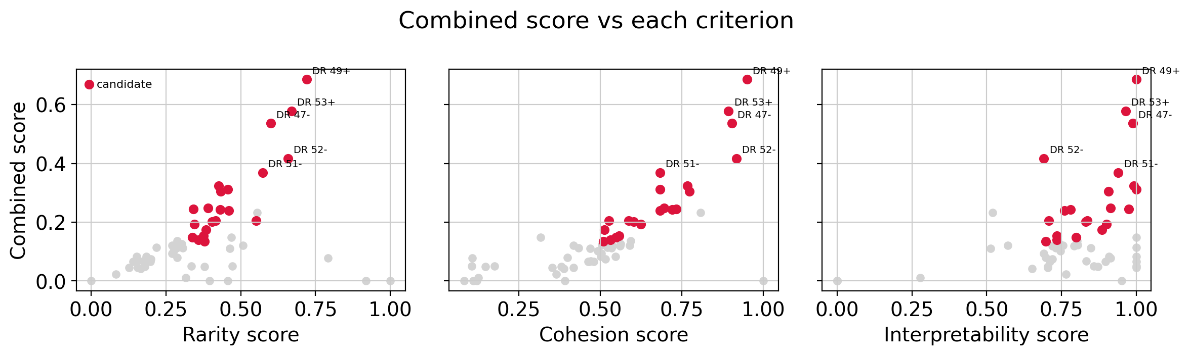
The combined score is the product of the three per-criterion scores, so we plot it against each one. Every dimension is shown; candidates (passing all three thresholds) are red, and the top 5 by combined score are labeled. A candidate scores highly on all three axes; a dimension weak on any single criterion is pulled down.

top5 = dim_stats.nlargest(5, "score")
components = [
    ("rarity_score", "Rarity score"),
    ("cohesion_score", "Cohesion score"),
    ("interpretability_score", "Interpretability score"),
]

cand = dim_stats[dim_stats["is_candidate"]]
noncand = dim_stats[~dim_stats["is_candidate"]]

fig, axes = plt.subplots(1, 3, figsize=(12, 3.6), sharey=True)
for ax, (col, label) in zip(axes, components):
    ax.scatter(noncand[col], noncand["score"], s=25, c="lightgray")
    ax.scatter(cand[col], cand["score"], s=35, c="crimson", label="candidate")
    for dim, r in top5.iterrows():
        ax.annotate(dim, (r[col], r["score"]), xytext=(4, 4), textcoords="offset points", fontsize=7)
    ax.set_xlabel(label)
axes[0].set_ylabel("Combined score")
axes[0].legend(frameon=False, fontsize=8, loc="upper left")
fig.suptitle("Combined score vs each criterion")
plt.tight_layout()
plt.show()

Which candidates are good rare-cell-type candidates?

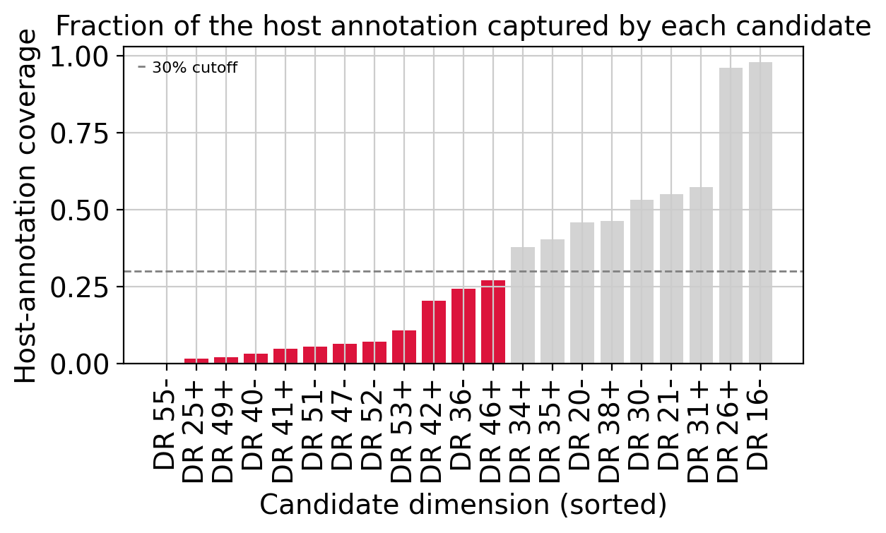
Now we bring in the existing annotation (final_annotation) — but the question is not whether a dimension’s active cells carry one label or several. A rare type whose cells are all labeled X is no more or less interesting than one labeled half X, half Y; both can be perfectly valid known types.

What signals a hidden population that needs refinement is different: the active cells are labeled X, yet they make up only a small fraction of all X cells (say < 30%). That means the dimension has carved out a distinct minority sub-population inside an existing annotation — a cell state the label does not resolve. So for each candidate we compute its host-annotation coverage: of all cells carrying the candidate’s dominant label, what fraction are active on this dimension.

• High coverage (≈100%) → the dimension simply re-discovers a known annotated type.

• Low coverage (< 30%) → a sub-population hidden inside that annotation — a refinement candidate.

# Now we finally subset to the candidates (all three criteria) and characterize them by annotation.
candidates = dim_stats[dim_stats["is_candidate"]].copy()

annotation = embed.obs[CELL_TYPE_COL].astype(str).values
annotation_totals = pd.Series(annotation).value_counts()


def host_annotation_coverage(embed, dim_title_direction, annotation, annotation_totals):
    """Dominant label of the active cells, and the fraction of *all* cells with that label
    that this dimension captures."""
    active = active_mask(embed, dim_title_direction)
    counts = pd.Series(annotation[active]).value_counts()
    host = counts.index[0]
    return host, counts.iloc[0] / annotation_totals[host]


coverage = [host_annotation_coverage(embed, dim_title_direction, annotation, annotation_totals)
            for dim_title_direction in candidates.index]
candidates["host_annotation"] = [host for host, _ in coverage]
candidates["host_coverage"] = [cov for _, cov in coverage]

Sorting the candidates by host-annotation coverage: dimensions on the right re-discover whole annotated types (e.g. one capturing nearly all Plasma cells, another nearly all pDCs), while those below the 30% cutoff are minority sub-populations hidden inside a label. The low-coverage candidates are the good rare-cell-type candidates — cell states the current annotation does not resolve.

cov_sorted = candidates.sort_values("host_coverage")
colors = ["crimson" if c < HOST_COVERAGE_CUTOFF else "lightgray" for c in cov_sorted["host_coverage"]]

fig, ax = plt.subplots(figsize=(max(5.0, 0.28 * len(cov_sorted)), 4))
ax.bar(cov_sorted.index, cov_sorted["host_coverage"], color=colors)
ax.axhline(HOST_COVERAGE_CUTOFF, ls="--", c="gray", lw=1, label=f"{HOST_COVERAGE_CUTOFF:.0%} cutoff")
ax.set_ylabel("Host-annotation coverage")
ax.set_xlabel("Candidate dimension (sorted)")
ax.set_title("Fraction of the host annotation captured by each candidate")
ax.tick_params(axis="x", rotation=90)
ax.legend(frameon=False, fontsize=8)
plt.tight_layout()
plt.show()

unannotated_candidates = candidates[candidates["host_coverage"] < HOST_COVERAGE_CUTOFF]
print(f"{len(unannotated_candidates)} unannotated candidates (host coverage < {HOST_COVERAGE_CUTOFF:.0%}).")
unannotated_candidates

12 unannotated candidates (host coverage < 30%).

	n_active	fraction_active	max_ood_score	cohesion	is_candidate	rarity_score	cohesion_score	interpretability_score	score	host_annotation	host_coverage
dim_title_direction
DR 49+	11	0.000339	10.000000	0.950921	True	0.720925	0.950921	1.000000	0.685543	HSPCs	0.021142
DR 53+	17	0.000523	7.863611	0.893626	True	0.670261	0.893626	0.965207	0.578123	Plasma cells	0.108527
DR 47-	31	0.000954	9.252443	0.903657	True	0.600341	0.903657	0.988752	0.536401	Monocyte-derived dendritic cells	0.064854
DR 52-	19	0.000585	1.186558	0.917455	True	0.657317	0.917455	0.691430	0.416973	Megakaryocyte progenitors	0.070370
DR 51-	39	0.001201	6.611657	0.682976	True	0.573623	0.682976	0.940103	0.368305	Monocyte-derived dendritic cells	0.054393
DR 42+	106	0.003263	10.000000	0.682977	True	0.457254	0.682977	1.000000	0.312294	Monocyte progenitors	0.203271
DR 41+	130	0.004002	5.237635	0.773856	True	0.433500	0.773856	0.906378	0.304060	NK cells	0.047515
DR 25+	189	0.005818	5.538980	0.695459	True	0.389948	0.695459	0.914477	0.248000	CD4+ T cells	0.016620
DR 46+	133	0.004094	2.203845	0.720604	True	0.430845	0.720604	0.781060	0.242495	Monocyte-derived dendritic cells	0.269874
DR 55-	47	0.001447	1.327584	0.527321	True	0.551907	0.527321	0.707687	0.205960	CD4+ T cells	0.002997
DR 36-	168	0.005172	3.123841	0.603192	True	0.403656	0.603192	0.831563	0.202471	Monocyte progenitors	0.242991
DR 40-	207	0.006372	1.235535	0.509244	True	0.379361	0.509244	0.697285	0.134706	CD14+ Monocytes	0.031398

Inspect the good candidates

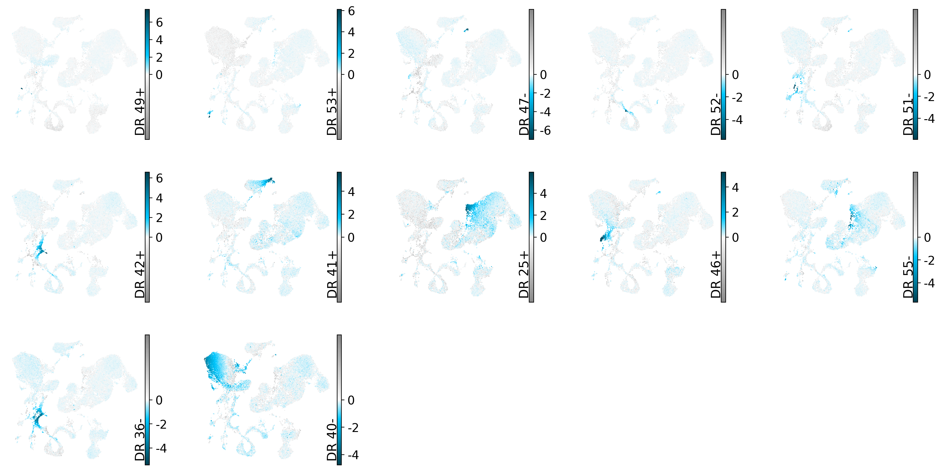
For every good rare-cell-type candidate we look at where its active cells sit in the latent UMAP and which genes define it. Each candidate should light up a small, coherent region (cohesion) with a distinct gene program (interpretability).

candidate_dims = unannotated_candidates.index.to_list()
drvi.utils.pl.plot_latent_dims_in_umap(embed, dim_subset=candidate_dims, directional=True, ncols=5)

# `interpretability_df` (from get_interpretability_scores) already holds the gene x dimension scores;
# we plot it directly with the utility function.
drvi.utils.pl.plot_interpretability_scores(interpretability_df, dim_subset=candidate_dims)

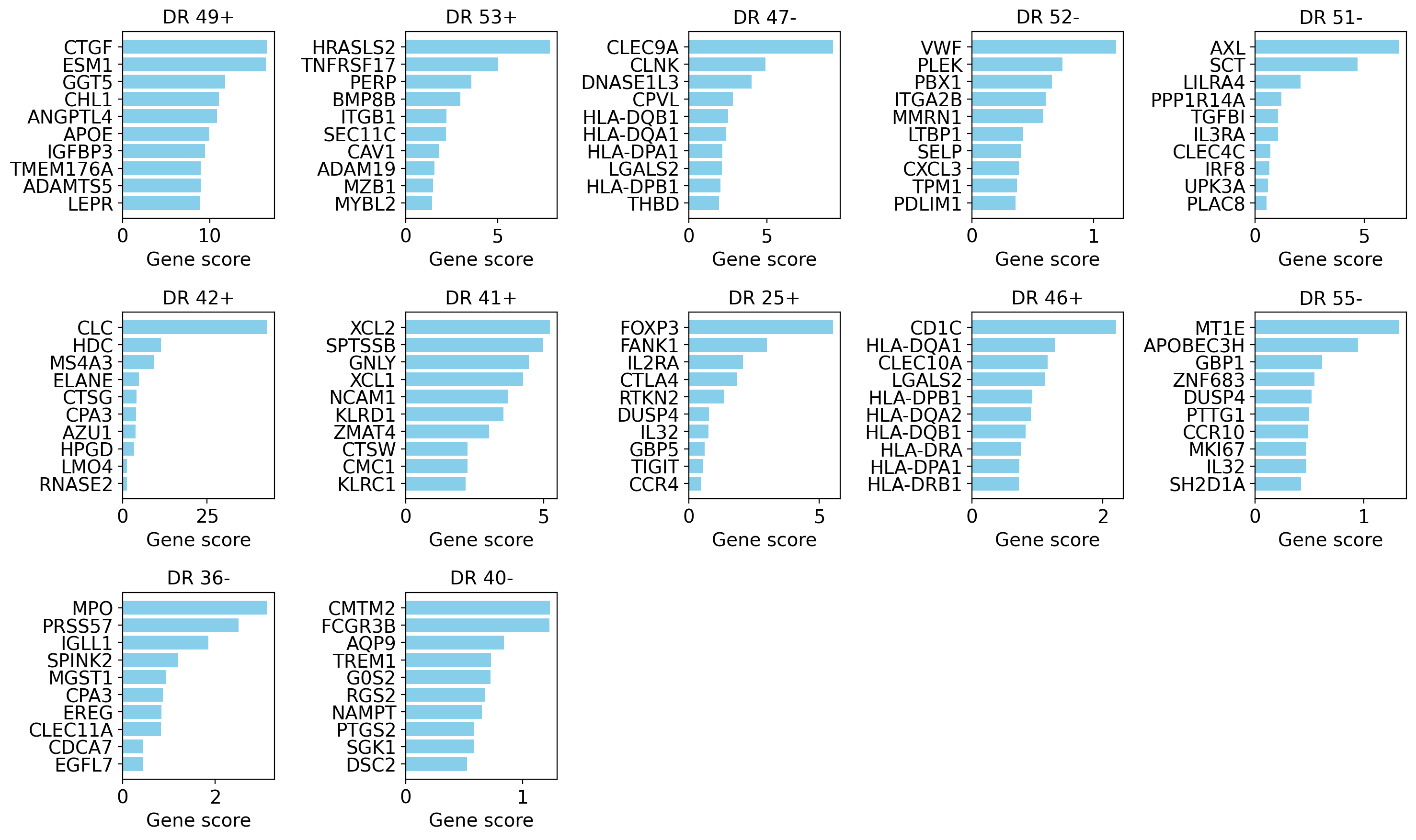
The candidates above represent rare cell types or substantially finer subclusters than the existing annotations. These subsets can usually be identified from their top marker genes.

A closer look: discovering the fibroblasts

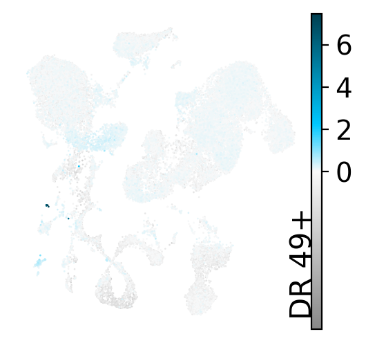
Among the candidates, the rarest one stands out: a tiny dimension (about a dozen cells) whose cells are filed under HSPCs yet are only ~2% of all HSPCs. Let us follow it end-to-end — identify it, read its gene program, and prove what it is.

novel_dim = unannotated_candidates["fraction_active"].idxmin()   # signed title of the rarest unannotated candidate
novel = unannotated_candidates.loc[novel_dim]
print(f"Rarest candidate: {novel_dim} "
      f"({int(novel['n_active'])} active cells, "
      f"filed under '{novel['host_annotation']}' = {novel['host_coverage']:.0%} of that label)")

Rarest candidate: DR 49+ (11 active cells, filed under 'HSPCs' = 2% of that label)

Where do these cells sit in the latent UMAP, and what gene program defines the dimension?

drvi.utils.pl.plot_latent_dims_in_umap(embed, dim_subset=[novel_dim], directional=True)

# Top genes of the dimension from the OOD interpretability scores computed earlier.
top_genes = interpretability_df[novel_dim].sort_values(ascending=False).head(15)
top_genes

index
CTGF        16.571638
ESM1        16.453249
GGT5        11.744926
CHL1        11.075065
ANGPTL4     10.839224
APOE         9.956368
IGFBP3       9.464329
TMEM176A     8.986178
ADAMTS5      8.935861
LEPR         8.833095
PCOLCE       8.585528
TNFAIP6      8.509926
APOD         8.253371
CYP1B1       8.215649
SOCS3        7.993901
Name: DR 49+, dtype: float32

drvi.utils.pl.plot_interpretability_scores(interpretability_df, dim_subset=[novel_dim])

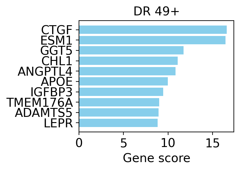
The program is dominated by extracellular-matrix / stromal genes — CTGF (CCN2), PCOLCE, ADAMTS5, IGFBP3, APOD, ANGPTL4 — none of which belong to immune cells. The hypothesis is clear: these few cells are fibroblasts, a stromal contaminant that the annotation merged into HSPCs.

Crucially, the canonical fibroblast marker COL1A1 is not in the 2000 HVGs, so the model never saw it. That makes it a perfect independent test of the hypothesis.

Validate with the held-out marker COL1A1

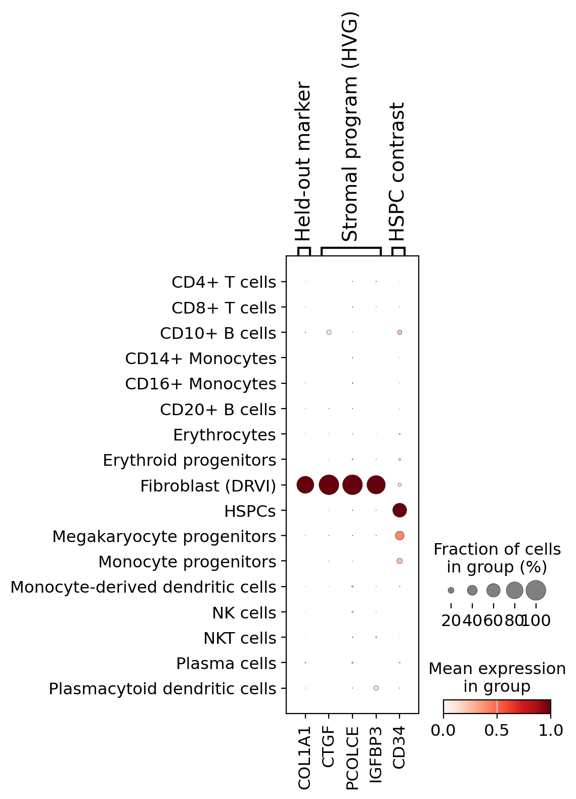
We load the full gene set, label the active cells of the novel dimension as Fibroblast (DRVI), and show that COL1A1 lights up specifically in this group — and not in the HSPCs they were mislabeled as.

# The full matrix (~2 GB) is only needed here.
full = sc.read(
    full_anndata_path,
    backup_url="https://exampledata.scverse.org/scvi-tools/Immune_ALL_human.h5ad",
)
full = full[embed.obs_names].copy()

assert "COL1A1" not in adata.var_names, "COL1A1 should be held out from the HVGs the model trained on"
assert "COL1A1" in full.var_names, "COL1A1 must be present in the full gene set"

# Ensure a log-normalized layer for the dotplot.
full.layers["log1p"] = full.layers["counts"].copy()
full.X = full.layers["log1p"]
sc.pp.normalize_total(full)
sc.pp.log1p(full)
full.layers["log1p"] = full.X.copy()

# Label the active cells of the novel dimension; everyone else keeps their original annotation.
active_novel = active_mask(embed, novel_dim)
full.obs["new_cell_type"] = np.where(
    active_novel, "Fibroblast (DRVI)", full.obs[CELL_TYPE_COL].astype(str)
)
print(full.obs["new_cell_type"].value_counts().loc[["Fibroblast (DRVI)"]])

new_cell_type
Fibroblast (DRVI)    11
Name: count, dtype: int64

Marker dotplot. COL1A1 is the held-out proof; the stromal HVG genes are the program DRVI used; CD34 is shown as a contrast marker for the HSPCs these cells were labeled as.

marker_genes = {
    "Held-out marker": ["COL1A1"],
    "Stromal program (HVG)": ["CTGF", "PCOLCE", "IGFBP3"],
    "HSPC contrast": ["CD34"],
}
sc.pl.dotplot(
    full,
    marker_genes,
    groupby="new_cell_type",
    standard_scale="var",
    layer="log1p",
    show=True,
)

Quantitative proof

col1a1 = np.asarray(
    full[:, "COL1A1"].layers["counts"].todense()
    if hasattr(full[:, "COL1A1"].layers["counts"], "todense")
    else full[:, "COL1A1"].layers["counts"]
).ravel()

frac_in_dim = (col1a1[active_novel] > 0).mean()
n_total_pos = int((col1a1 > 0).sum())
print(f"COL1A1+ among the {int(active_novel.sum())} cells of {novel_dim}: {frac_in_dim:.0%}")
print(f"COL1A1+ cells in the whole dataset: {n_total_pos} / {full.n_obs}")

COL1A1+ among the 11 cells of DR 49+: 82%
COL1A1+ cells in the whole dataset: 67 / 32484

A large majority of the dimension’s cells express COL1A1, while only ~70 cells express it across the entire dataset (of >32,000) — overwhelming, independent confirmation that DRVI isolated the fibroblasts.

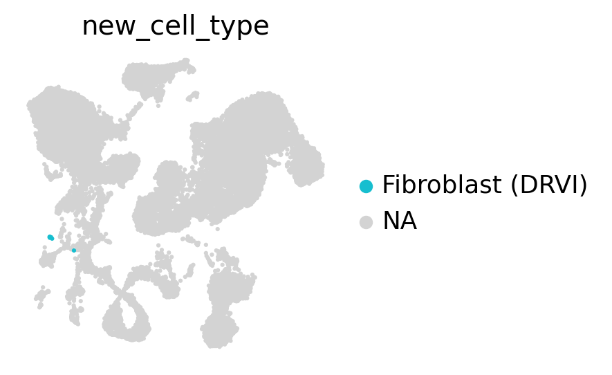
Where are the fibroblasts in the UMAP?

embed.obs["new_cell_type"] = full.obs["new_cell_type"].values
sc.pl.umap(embed, color="new_cell_type", groups=["Fibroblast (DRVI)"], size=20, frameon=False)

Wrap-up

Rare, un-annotated populations surface in DRVI as dedicated latent dimensions. The recipe:

1. Rarity & interpretability — few active cells (|latent| past half the dimension’s peak) and a specific gene program (max OOD score > 1).

2. Spatial cohesion — the active cells form a tight blob on the UMAP (high UMAP cohesion).

3. Spot the ones needing refinement — candidates that capture only a small fraction (< 30%) of their host annotation are hidden sub-populations the labels do not resolve.

4. Propose an identity — read the dimension’s top interpretability genes.

5. Confirm it [optional] — with an independent, held-out marker (COL1A1 for fibroblasts here).

All thresholds (the activity cutoff, the rare-fraction, cohesion, OOD, and host-coverage cutoffs) are tunable. Here the activity cutoff is adaptive — half of each dimension’s peak |latent| (max(|value|) / 2), which self-calibrates per dimension; a fixed cutoff such as ±2 is a common alternative. The same recipe works for any rare population in any DRVI model — the immune fibroblasts are just a clean illustration.