General training and interpretability pipeline#
In this notebook, we analyze the immune dataset of 9 batches from four human peripheral blood and bone marrow studies, with 16 annotated cell types. We apply DRVI with 128 latent dimensions to showcase the following:
How to train DRVI
Observe vanished dimensions
Observe the latent space in UMAP and heatmap
How to run the interpretability pipeline
How to identify and check individual dimensions
Contact#
For questions and help requests, you can reach out in the scverse discourse.
If you found a bug, please use the issue tracker.
Install#
This notebook uses the tutorials extra of drvi-py (DRVI plus helper packages such as
leidenalg). Install it once in your environment with:
pip install "drvi-py[tutorials]"
On Colab, the next cell does this for you. Remove it if your environment is already set up.
import sys
import subprocess

# if branch is stable, will install via pypi, else will install from source
branch = "latest"
IN_COLAB = "google.colab" in sys.modules

if IN_COLAB and branch == "stable":
    subprocess.check_call([sys.executable, "-m", "pip", "install", "drvi-py[tutorials]"])
elif IN_COLAB and branch != "stable":
    subprocess.check_call([sys.executable, "-m", "pip", "install",
                           "git+https://github.com/theislab/drvi.git#egg=drvi-py[tutorials]"])
Imports#
import warnings
warnings.filterwarnings("ignore")
import anndata as ad
import scanpy as sc

import scvi
import drvi
from pathlib import Path
from drvi.model import DRVI
print("Last run with scvi-tools version:", scvi.__version__)
print("Last run with DRVI version:", drvi.__version__)
Last run with scvi-tools version: 1.4.3
Last run with DRVI version: 0.2.6
# Making plots prettier
sc.settings.set_figure_params(dpi=100, frameon=False)
sc.set_figure_params(dpi=100)
sc.set_figure_params(figsize=(3, 3))

from matplotlib import pyplot as plt
plt.rcParams["figure.dpi"] = 100
plt.rcParams["figure.figsize"] = (3, 3)
Config#
# Set this to false if you already trained your model and do not want to retrain.
overwrite = False
SEED = 1  # Set to None if you don't want to set seed

# Set input output directory to load data from and store model and embeddings there
# We use tmp_io/ directory in the same place as this notebook. Update accordingly.
io_dir = Path("./tmp_io/drvi_immune_128/")
io_dir.mkdir(parents=True, exist_ok=True)
io_dir
PosixPath('tmp_io/drvi_immune_128')
Download and load data#
We use the immune dataset (SCIB, Luecken et al.) hosted on the scverse example data server. The Villani
batch is already removed because it contains non-count values, and 2000 batch-aware highly variable
genes are already selected.
input_anndata_path = io_dir.parent / "Immune_HVG_human.h5ad"
adata = sc.read(
    input_anndata_path,
    backup_url="https://exampledata.scverse.org/scvi-tools/Immune_HVG_human.h5ad",
)
adata
AnnData object with n_obs × n_vars = 32484 × 2000
    obs: 'batch', 'chemistry', 'data_type', 'dpt_pseudotime', 'final_annotation', 'mt_frac', 'n_counts', 'n_genes', 'sample_ID', 'size_factors', 'species', 'study', 'tissue'
    uns: 'batch_colors', 'final_annotation_colors', 'log1p', 'neighbors', 'pca', 'umap'
    obsm: 'X_pca', 'X_umap'
    varm: 'PCs'
    layers: 'counts'
    obsp: 'connectivities', 'distances'
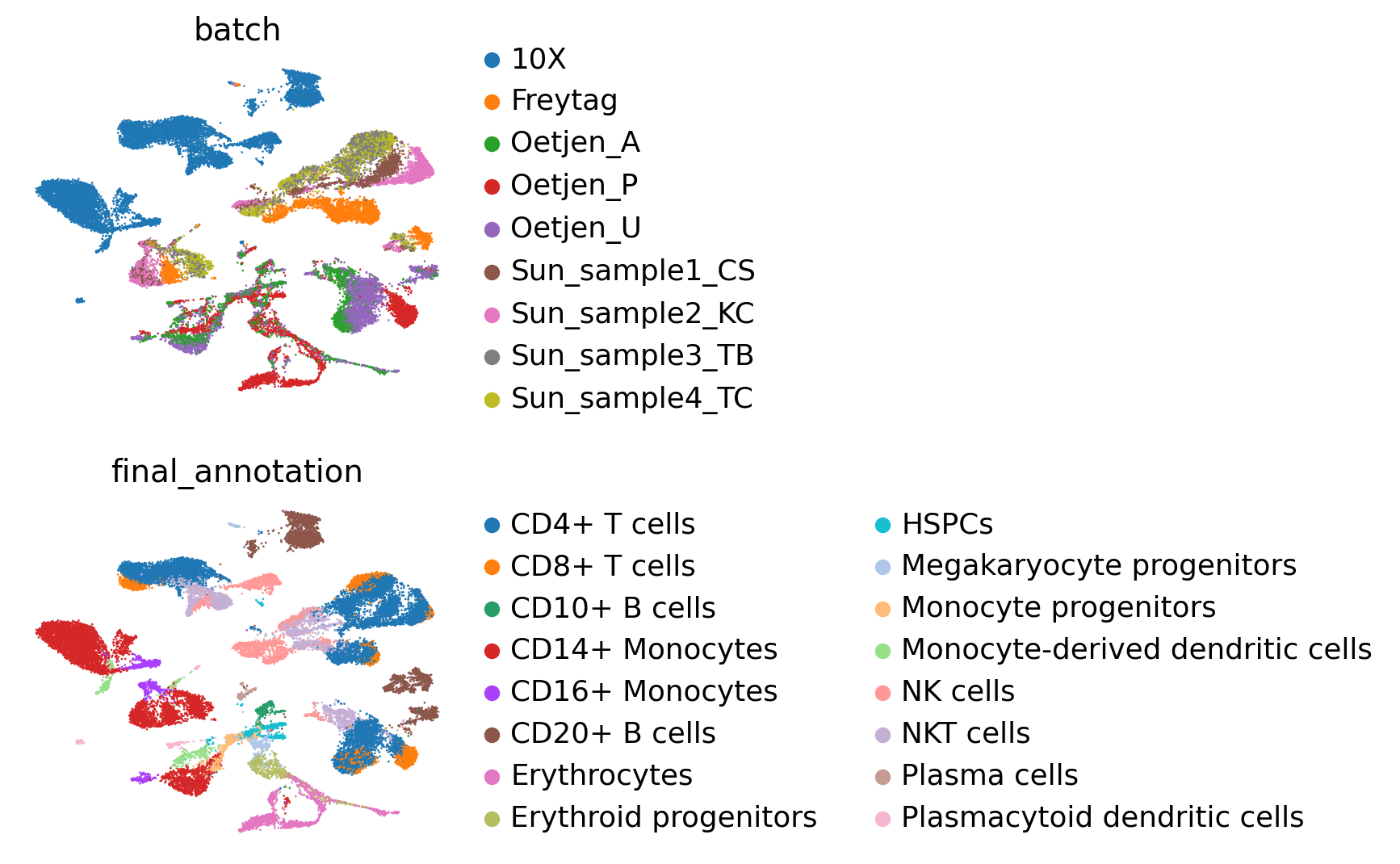
sc.pl.umap(adata, color=["batch", "final_annotation"], ncols=1, frameon=False)
Train DRVI#
# You can also skip this cell if model is already trained

# Setup data
DRVI.setup_anndata(
    adata,
    # DRVI accepts count data by default.
    # Do not forget to change gene_likelihood if you provide a non-count data.
    layer="counts",
    batch_key="batch",
    # In addition to batch_key, you can also provide additional `categorical_covariate_keys`.
    # DRVI accepts count data by default.
    # Set to false if you provide log-normalized data and use normal distribution (mse loss).
    is_count_data=True,
)

# Setting seed (set to None if you don't want to fix seed)
scvi.settings.seed = SEED

# construct the model
model = DRVI(
    adata,
    n_latent=128,
    # For encoder and decoder dims, provide a list of integers.
    encoder_dims=[128, 128],
    decoder_dims=[128, 128],
    # depending on the variability of gene dispersions use 'gene' (default) or 'gene-batch'
    # dispersion='gene',
    # dispersion='gene-batch',
)
model
INFO DRVI: The model has been initialized
DRVI
Latent size: 128, splits: 128, pooling of splits: 'logsumexp',
Encoder dims: [128, 128],
Decoder dims: [128, 128],
Gene likelihood: pnb,

Training status: Not Trained
# For cpu training you should add the following line to the model.train parameters:
# accelerator="cpu", devices=1,
#
# For mps acceleration on macbooks, add the following line to the model.train parameters:
# accelerator="mps", devices=1,
#
# For gpu training don't provide any additional parameter.
# More details here: https://lightning.ai/docs/pytorch/stable/accelerators/gpu_basic.html

n_epochs = 400
model_path = io_dir / "drvi_model"

# train the model and save (if not already trained)
if overwrite or not model_path.exists():
    model.train(
        max_epochs=n_epochs,
        early_stopping=False,
        early_stopping_patience=20,
        # mps
        # accelerator="mps", devices=1,
        # cpu
        # accelerator="cpu", devices=1,
        # gpu: no additional parameter
        #
        # No need to provide `plan_kwargs` if n_epochs >= 400.
        plan_kwargs={
            "n_epochs_kl_warmup": n_epochs,
        },
    )

    # Save the model
    model.save(model_path, overwrite=True)

# Runtime:
# The runtime for CPU laptop (M1) is 208 minutes
# The runtime for Macbook gpu (M1) is 64 minutes
# The runtime for GPU (H100) is 10 minutes
Latent space#
# Load the model
model = DRVI.load(model_path, adata)
model
INFO     File tmp_io/drvi_immune_128/drvi_model/model.pt already downloaded
INFO     DRVI: The model is trained with DRVI version 0.2.6.
INFO     DRVI: Updaging data setup config ...
INFO     DRVI: Done updating data source registry. Loading in DRVI version 0.2.6.
INFO     DRVI: Loading model from DRVI version 0.2.6.
INFO     DRVI: Done updating model args. Loading in 0.2.6.
INFO     DRVI: The model has been initialized
DRVI
Latent size: 128, splits: 128, pooling of splits: 'logsumexp',
Encoder dims: [128, 128],
Decoder dims: [128, 128],
Gene likelihood: pnb,

Training status: Trained
embed_path = io_dir / "embed.h5ad"

# Create latent space data in anndata format
if overwrite or not embed_path.exists():
    embed = ad.AnnData(model.get_latent_representation(), obs=adata.obs)

    # We set latent dimension stats here (see docs for more info)
    print("Setting latent dimension stats ...")
    model.set_latent_dimension_stats(embed, vanished_threshold=0.5)

    # We immediately calculate the interpretability gene scores with different approaches
    print("Calculating gene scores per factor ...")
    # out-of-distribution (OOD) approach uses decoder reconstructions to calculate gene scores (faster)
    model.calculate_interpretability_scores(embed, "OOD")
    # within-distribution (IND) approach iterates over all cells and calculates gene scores
    model.calculate_interpretability_scores(embed, "IND")

    print("Dimension reduction ...")
    sc.pp.neighbors(embed, n_neighbors=10, use_rep="X", n_pcs=embed.X.shape[1])
    sc.tl.umap(embed, spread=1.0, min_dist=0.5, random_state=123)
    sc.pp.pca(embed)

    print("Writing ...")
    embed.write_h5ad(embed_path)
Setting latent dimension stats ...
Calculating gene scores per factor ...
INFO     DRVI: Using all 9 combinations of batch and categorical covariates.
Dimension reduction ...
Writing ...
embed = sc.read_h5ad(embed_path)
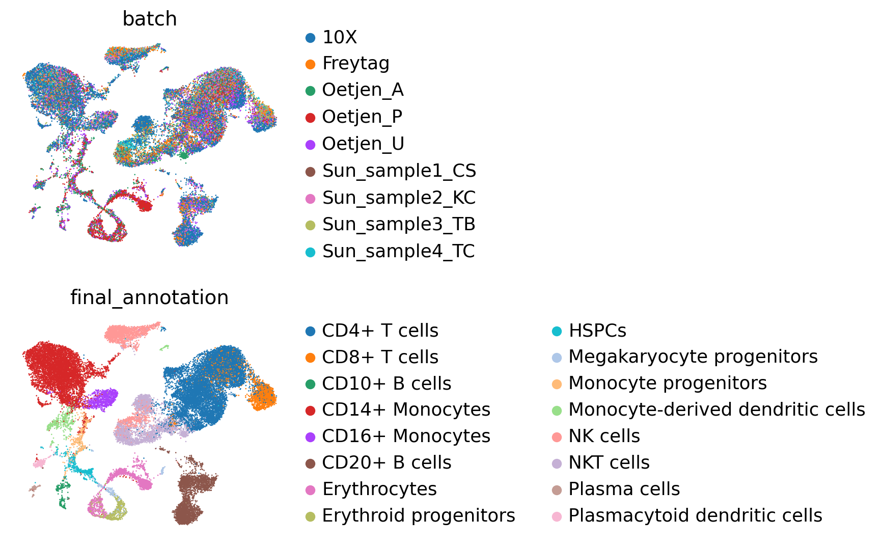
sc.pl.umap(embed, color=["batch", "final_annotation"], ncols=1, frameon=False)
Check latent dimension stats#
# Show information for latent factors
embed.var.sort_values("reconstruction_effect", ascending=False)[:5]
| original_dim_id | reconstruction_effect | order | max_value | mean | min | max | std | std_abs | title | vanished | vanished_positive_direction | vanished_negative_direction | |
|---|---|---|---|---|---|---|---|---|---|---|---|---|---|
| 46 | 46 | 43952664.0 | 0 | 2.673029 | -0.119346 | -2.673029 | 1.941184 | 0.937229 | 0.458564 | DR 1 | False | False | False |
| 86 | 86 | 12391402.0 | 1 | 3.987986 | 0.016858 | -3.987986 | 1.772654 | 0.894534 | 0.581306 | DR 2 | False | False | False |
| 33 | 33 | 9010006.0 | 2 | 4.408394 | -0.061179 | -2.167124 | 4.408394 | 0.777968 | 0.606769 | DR 3 | False | False | False |
| 118 | 118 | 7411521.5 | 3 | 3.799625 | -0.034869 | -3.799625 | 1.851009 | 0.809966 | 0.526571 | DR 4 | False | False | False |
| 71 | 71 | 6725966.0 | 4 | 4.177349 | 0.029957 | -1.048303 | 4.177349 | 0.674260 | 0.583410 | DR 5 | False | False | False |
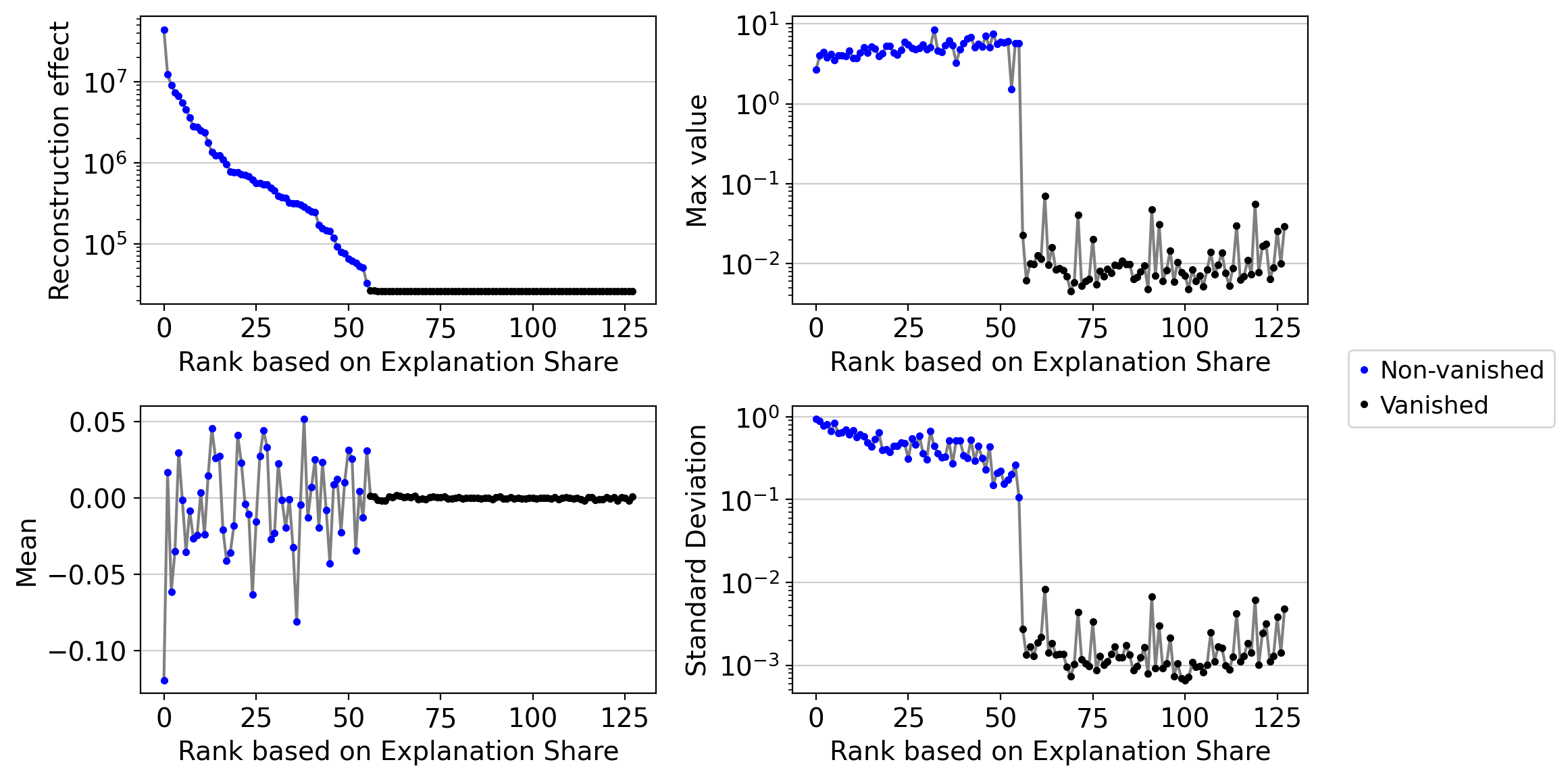
drvi.utils.pl.plot_latent_dimension_stats(embed, ncols=2)
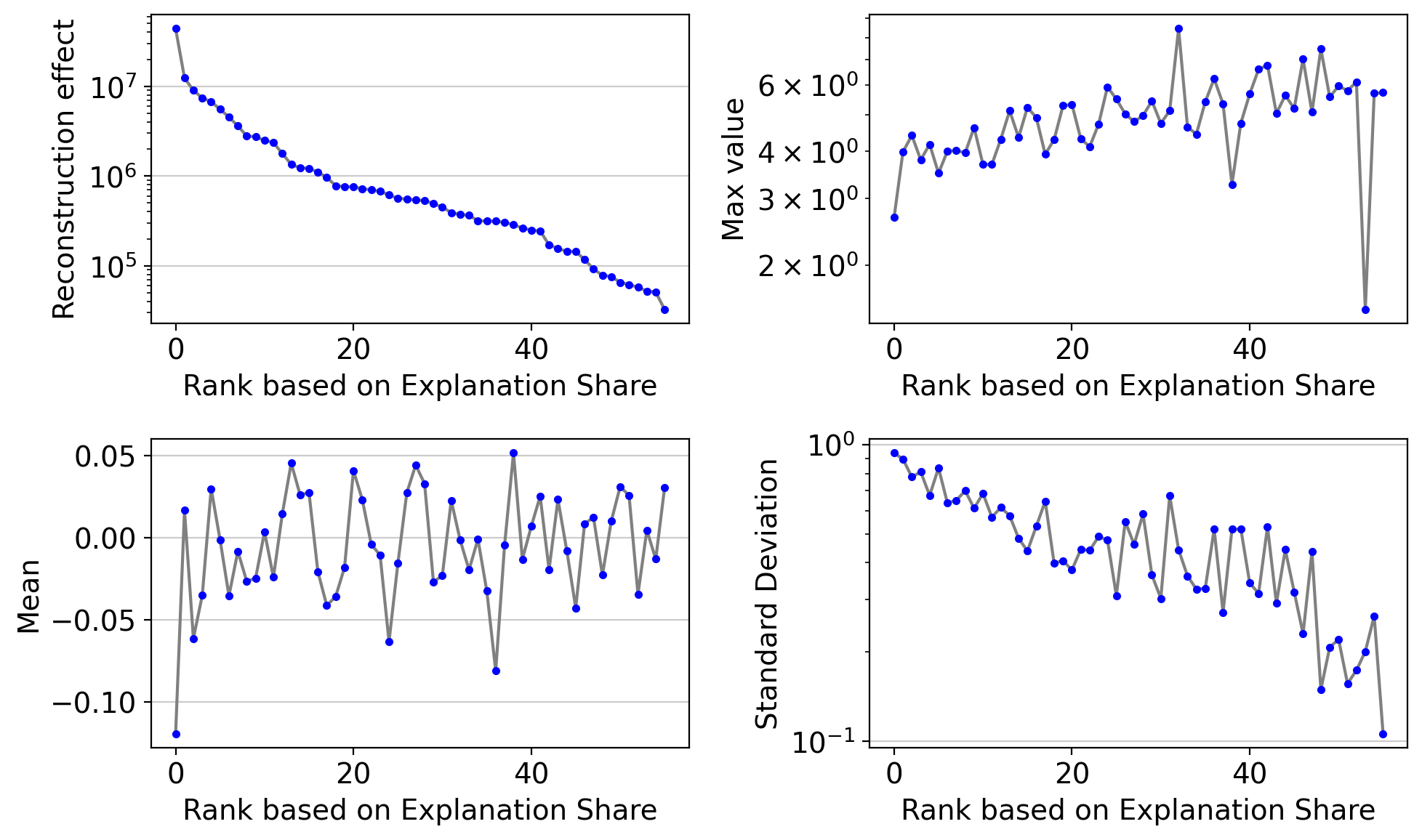
You can check the same plot after removing vanished dimensions
drvi.utils.pl.plot_latent_dimension_stats(embed, ncols=2, remove_vanished=True)
Plot latent dimensions#
By default, vanished dimensions are not plotted. Change arguments if you would like to.
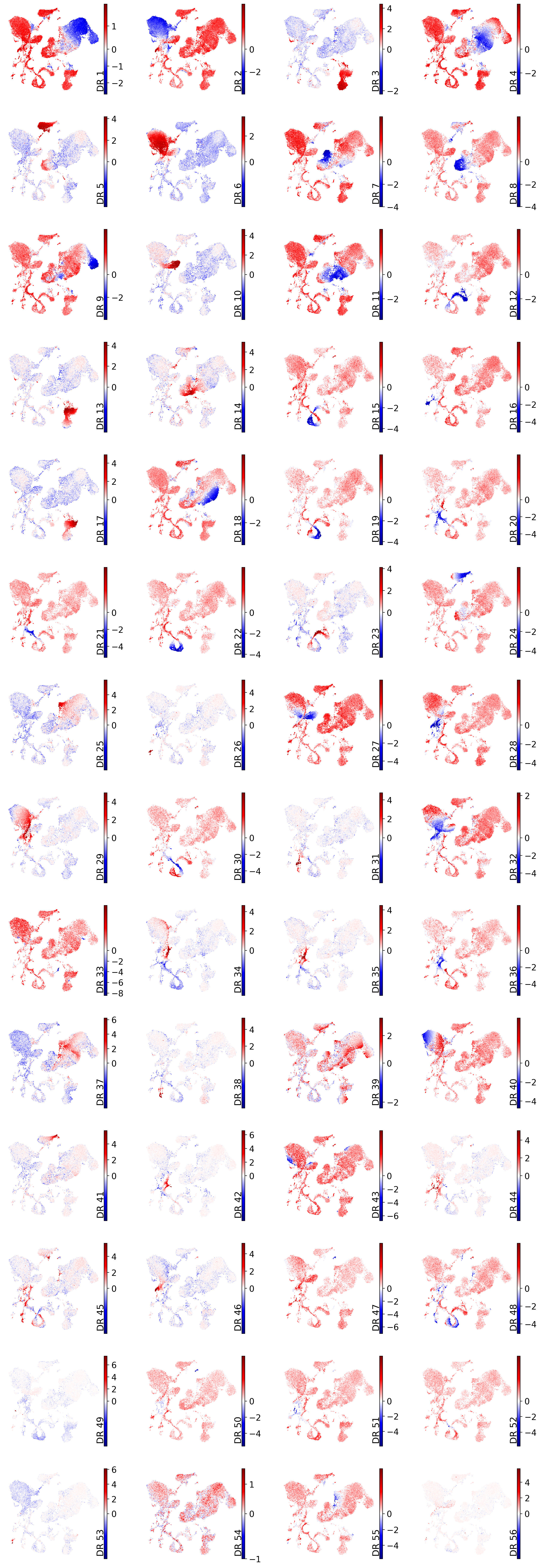
UMAP#
drvi.utils.pl.plot_latent_dims_in_umap(embed)
Heatmap#
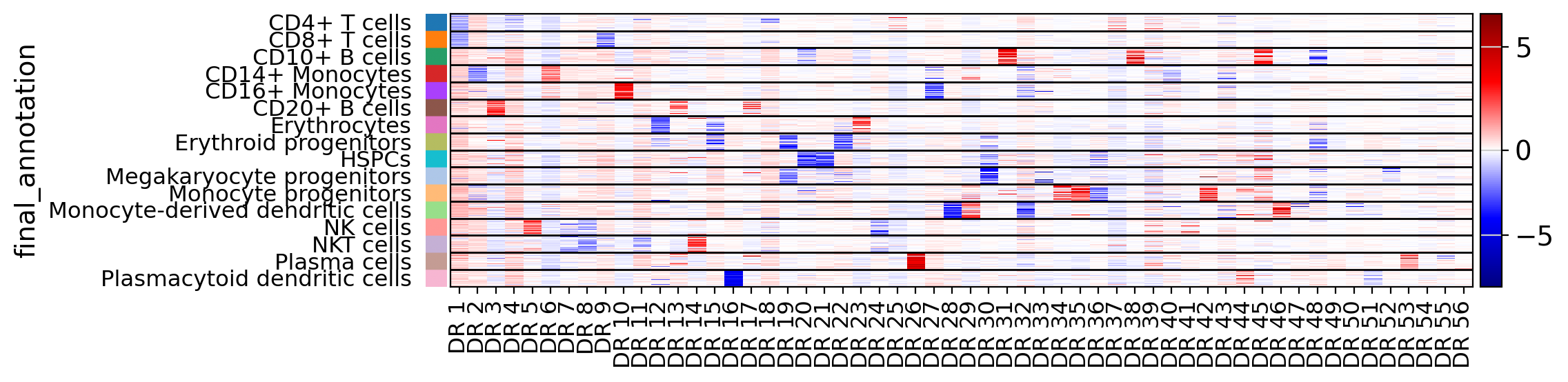
Heatmaps can be useful to visualize general relationship between latent dims and known categories of data
drvi.utils.pl.plot_latent_dims_in_heatmap(embed, "final_annotation", title_col="title")
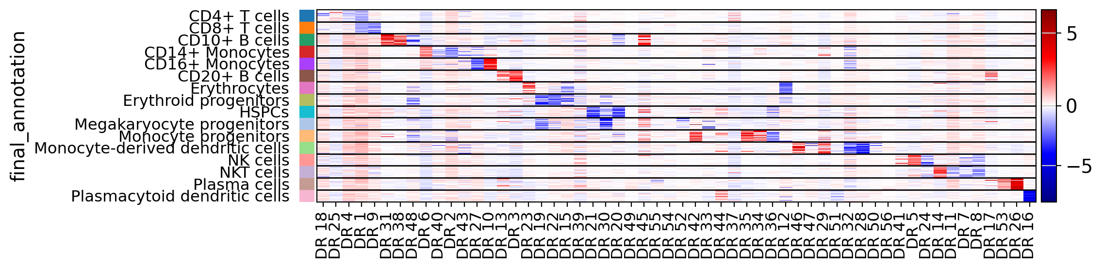
It is possible to sort dimensions based on the top relevance with respect to a categorical variable
drvi.utils.pl.plot_latent_dims_in_heatmap(embed, "final_annotation", title_col="title", sort_by_categorical=True)
Interpretability#
The scores are already calculated and stored in embed.varm.
embed.varm
AxisArrays with keys: IND_exp_weighted_mean_negative, IND_exp_weighted_mean_positive, IND_linear_weighted_mean_negative, IND_linear_weighted_mean_positive, IND_max_negative, IND_max_positive, OOD_combined_negative, OOD_combined_positive, OOD_max_possible_negative, OOD_max_possible_positive, OOD_min_possible_negative, OOD_min_possible_positive, PCs
Out-Of-Distribution (OOD) scores#
This approach iterates over latent dimensions and calculates decoder effects.
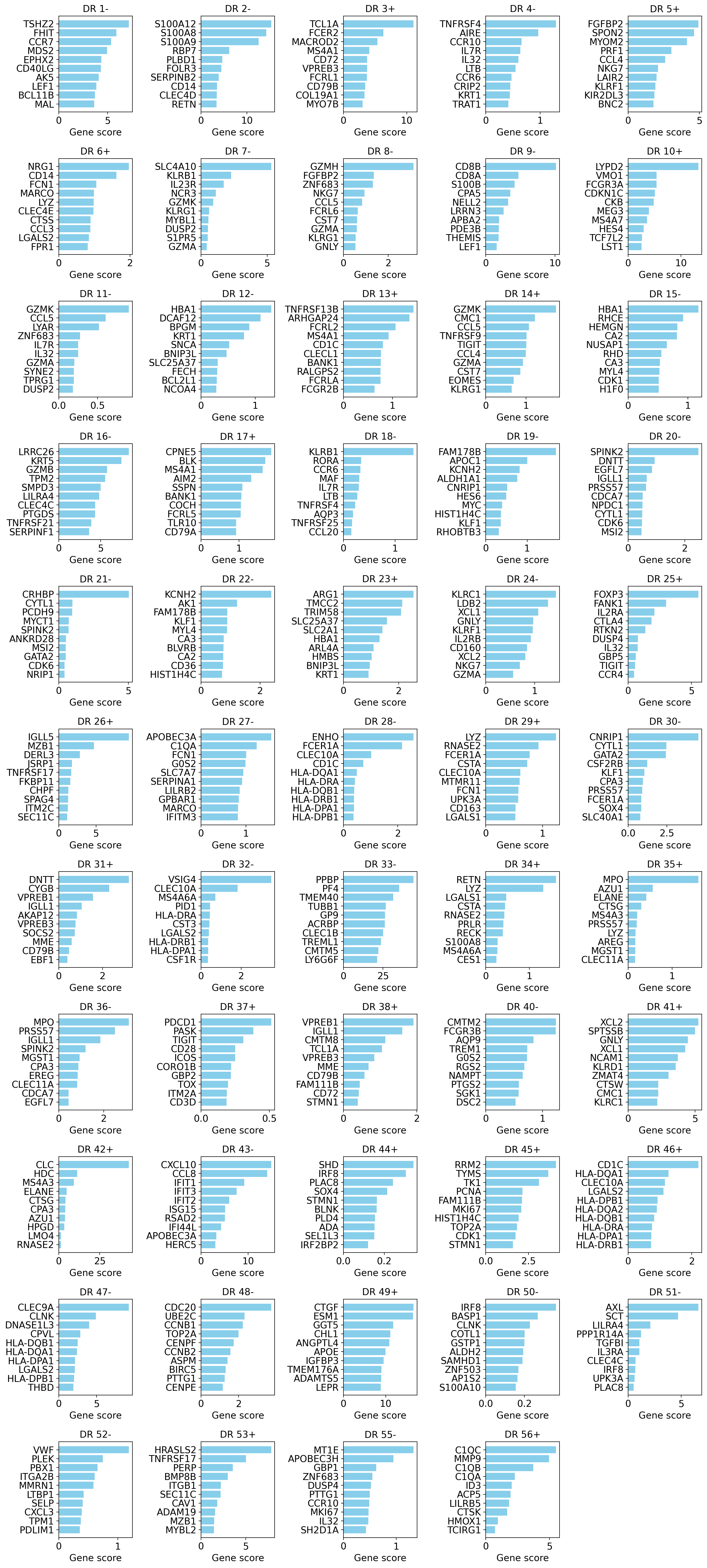
We first visualize gene scores based on default algorithm (optionally you can pass key="OOD_combined")
These scores show a combination of max effect and specificity. So, this is our suggested method to consider for finding cell-types and most specific genes of a program.
If human readable gene symbols are present in a different column of adata other than adata.var.index, please pass that column as gene_symbols=... to the function.
model.plot_interpretability_scores(embed, adata)
You can get all scores as a dataframe:
# Note: Genes (rows of the dataframe) appear as in adata and are not sorted.
scores_df = model.get_interpretability_scores(embed, adata)
scores_df.iloc[:10, :10]
| title | DR 1+ | DR 1- | DR 2+ | DR 2- | DR 3+ | DR 3- | DR 4+ | DR 4- | DR 5+ | DR 5- |
|---|---|---|---|---|---|---|---|---|---|---|
| index | ||||||||||
| TCL1A | 0.000000e+00 | 0.009215 | 5.813187e-11 | 0.000651 | 11.079925 | 1.764167e-10 | 2.854803e-11 | 0.000547 | 0.000348 | 0.000000e+00 |
| IGLL5 | 0.000000e+00 | 0.001222 | 0.000000e+00 | 0.000468 | 0.434816 | 0.000000e+00 | 0.000000e+00 | 0.000181 | 0.000018 | 6.745419e-12 |
| PTGDS | 0.000000e+00 | 0.001911 | 1.868569e-08 | 0.000612 | 0.000071 | 3.509566e-08 | 0.000000e+00 | 0.005746 | 0.469179 | 1.019392e-10 |
| GZMB | 3.417426e-10 | 0.020154 | 2.159570e-09 | 0.001463 | 0.003298 | 1.036622e-08 | 2.067888e-09 | 0.001405 | 1.692503 | 4.650348e-09 |
| PPBP | 5.485011e-10 | 0.000645 | 2.178695e-09 | 0.000501 | 0.000208 | 2.160353e-09 | 5.194226e-10 | 0.000028 | 0.000078 | 4.936434e-09 |
| CD79A | 5.760133e-12 | 0.014575 | 2.063214e-09 | 0.001043 | 2.554360 | 2.228262e-10 | 1.207860e-10 | 0.001227 | 0.000167 | 1.087898e-07 |
| FGFBP2 | 2.148176e-10 | 0.031997 | 1.850519e-09 | 0.000414 | 0.008896 | 1.674986e-09 | 7.094564e-10 | 0.001269 | 4.922354 | 4.795854e-09 |
| FCGR3A | 8.817046e-11 | 0.014633 | 1.007646e-07 | 0.004702 | 0.001230 | 1.522646e-10 | 8.617462e-11 | 0.000321 | 0.740610 | 3.888595e-10 |
| GNLY | 2.291421e-10 | 0.036005 | 1.976913e-09 | 0.002981 | 0.011447 | 1.869567e-08 | 2.071374e-10 | 0.005043 | 1.684550 | 3.476645e-09 |
| GZMH | 5.015358e-10 | 0.044191 | 1.972517e-09 | 0.002572 | 0.006846 | 2.701932e-09 | 2.072612e-09 | 0.000669 | 1.280149 | 2.901617e-09 |
A user can take a deeper look into individual dimensions. By visualizing the min_possible, and max_possible log-fold-changes of each dimension in OOD settings. Please refer to paper appendix for details on these scores that together form OOD_combined.
scores_df = model.get_interpretability_scores(embed, adata, key="OOD_max_possible")
scores_df = model.get_interpretability_scores(embed, adata, key="OOD_min_possible")
or for visualization:
model.plot_interpretability_scores(embed, adata, key="OOD_max_possible")
model.plot_interpretability_scores(embed, adata, key="OOD_min_possible")
Users can plot top relevant genes of a factor on UMAP using scanpy plotting functions:
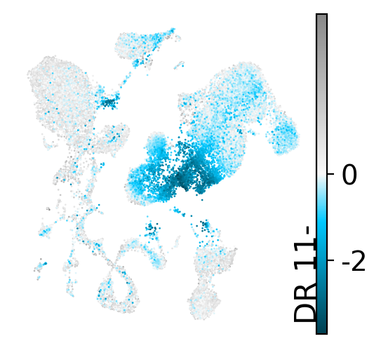
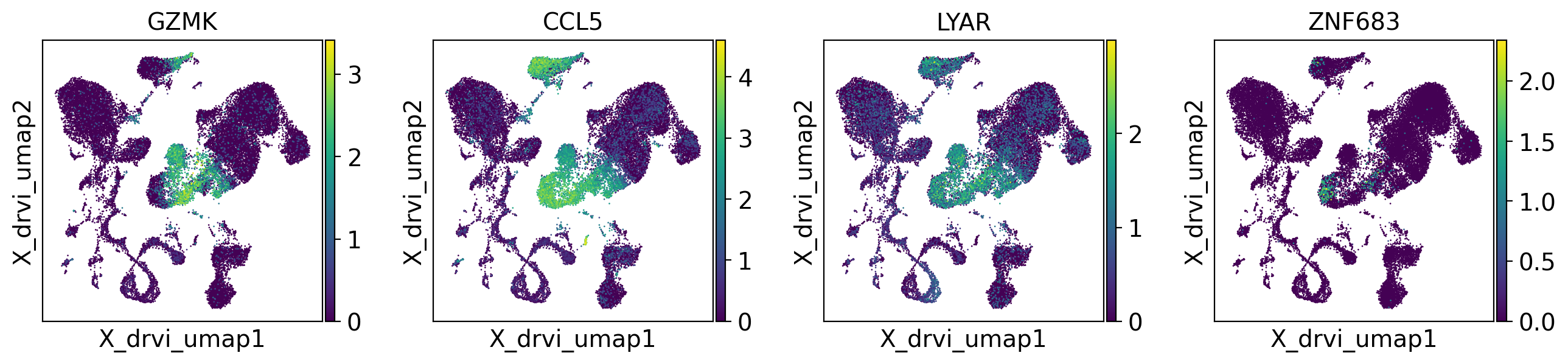
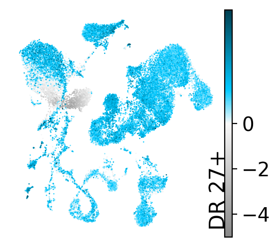
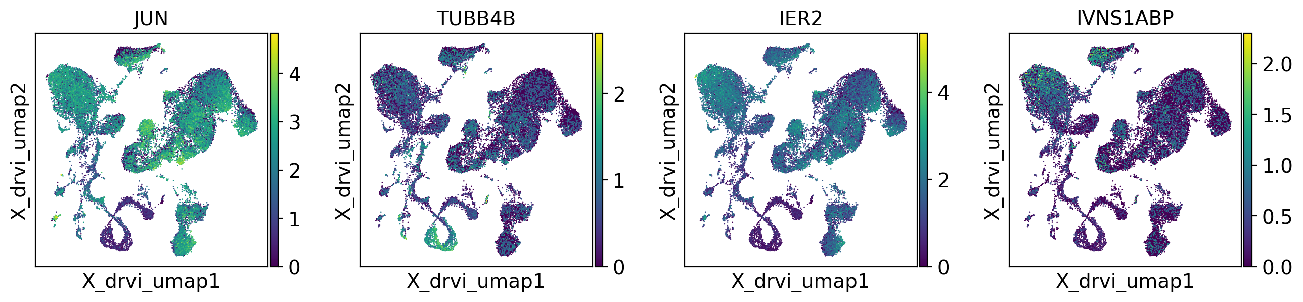
# DR 11- shows CD8+ cells and DR 27+ shows T-reg (May vary depending on the system and initialization)

# We first copy UMAP embeddings to original anndata
adata.obsm['X_drvi_umap'] = embed[adata.obs.index].obsm['X_umap']

# Show top 4 genes related to these two dimensions
for dim_title in ['DR 11-', 'DR 27+']:
    print(dim_title)
    top_genes = scores_df[dim_title].sort_values(ascending=False).index.to_list()[:4]
    drvi.utils.pl.plot_latent_dims_in_umap(embed, dim_subset=[dim_title], directional=True)
    sc.pl.embedding(adata, "X_drvi_umap", color=top_genes)
DR 11-
DR 27+
Within-Distribution (IND) scores#
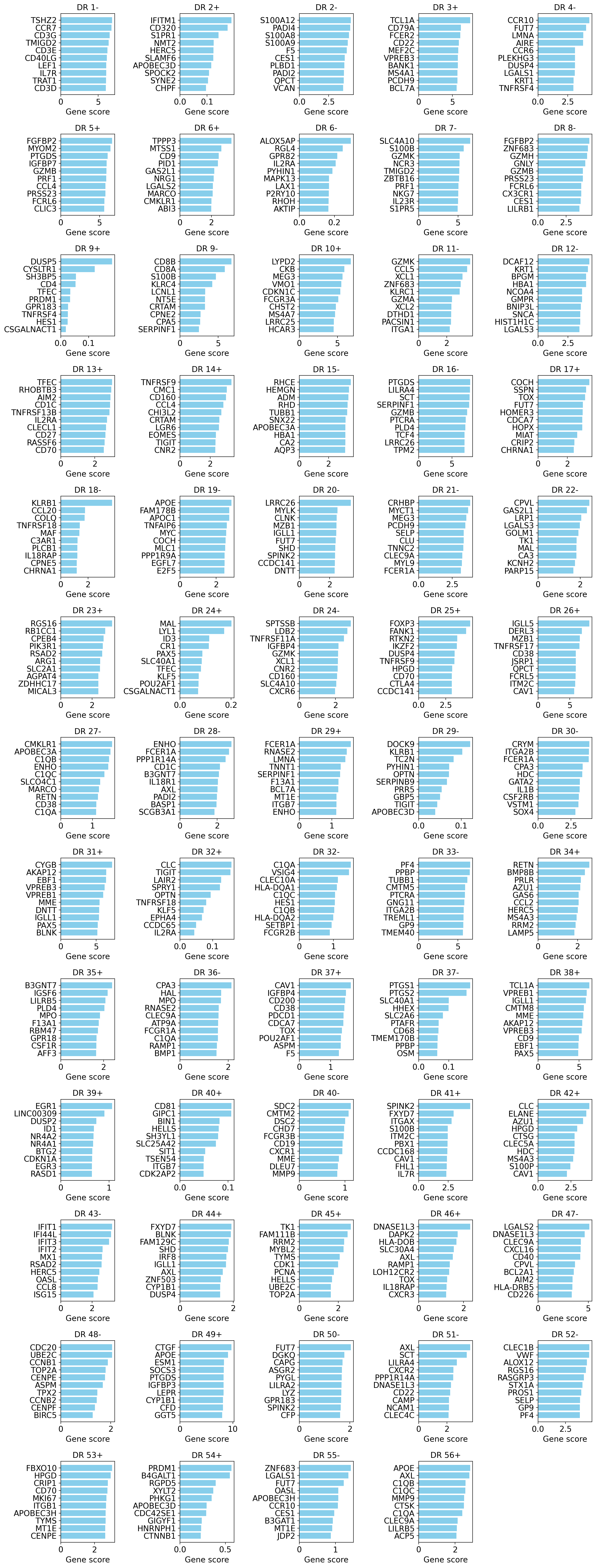
This approach iterates over all cells in anndata and averages the effect of each latent factor on each gene. The scores are already stored in embed.
These scores reflect the broad mechanistic effect of each latent dimension. Because genes are not filtered for uniqueness, shared genes retain high scores, providing a complete view of how each factor influences the genetic landscape.
model.plot_interpretability_scores(embed, adata, key="IND_linear_weighted_mean")
You can get all scores as a dataframe:
# Note: Genes (rows of the dataframe) appear as in adata and are not sorted.
scores_df = model.get_interpretability_scores(embed, adata, key="IND_linear_weighted_mean")
scores_df.iloc[:10, :10]
| title | DR 1+ | DR 1- | DR 2+ | DR 2- | DR 3+ | DR 3- | DR 4+ | DR 4- | DR 5+ | DR 5- |
|---|---|---|---|---|---|---|---|---|---|---|
| index | ||||||||||
| TCL1A | 0.000220 | 2.780176 | 0.004233 | 1.078486 | 7.625378 | 0.000019 | 0.001314 | 1.134821 | 1.862824 | 9.422505e-06 |
| IGLL5 | 0.000006 | 2.523443 | 0.000938 | 0.818631 | 4.711336 | 0.000004 | 0.000348 | 1.081231 | 1.184789 | 3.985862e-07 |
| PTGDS | 0.000803 | 2.386094 | 0.016986 | 1.115268 | 0.555248 | 0.008169 | 0.000093 | 2.017383 | 6.056585 | 1.216210e-06 |
| GZMB | 0.000904 | 2.605211 | 0.006223 | 0.937901 | 1.765631 | 0.002894 | 0.002173 | 0.872495 | 5.896867 | 1.391243e-05 |
| PPBP | 0.005586 | 2.594714 | 0.002119 | 1.765077 | 1.574105 | 0.000740 | 0.001821 | 0.826368 | 1.234926 | 4.912070e-05 |
| CD79A | 0.000072 | 3.418418 | 0.004669 | 1.300531 | 6.274120 | 0.000012 | 0.000979 | 1.040811 | 1.536780 | 2.397711e-04 |
| FGFBP2 | 0.001066 | 2.953458 | 0.010106 | 0.536246 | 1.660775 | 0.000440 | 0.002087 | 0.831935 | 6.636801 | 1.521198e-06 |
| FCGR3A | 0.001004 | 2.588500 | 0.014295 | 1.056512 | 1.442250 | 0.000757 | 0.000920 | 0.628357 | 5.417796 | 7.495910e-06 |
| GNLY | 0.000316 | 2.623381 | 0.004296 | 1.255002 | 1.632082 | 0.005335 | 0.000101 | 1.177773 | 5.253168 | 2.497883e-06 |
| GZMH | 0.000757 | 2.265003 | 0.000711 | 0.820256 | 1.371268 | 0.000583 | 0.002756 | 0.607529 | 5.018300 | 2.212242e-06 |
Identification of programs#
Once we identify the top relevant genes, we can determine some programs through supervised external information, such as:
existing annotations
examination by biologists
gene-set enrichment analysis (GSEA)
scientific literature
automated tools based on language models
It is worth mentioning that since such supervised information is not given to the model, the quality of the derived signatures is neither affected nor biased by it. Unidentified processes with high gene scores are promising candidates for further literature search, additional analysis, and even experimental design.